Comparative Analysis of Horticultural Lighting Systems

Centered-Square COB LED System

COB LEDs (Samsung BXRE-30E6500-C-83) are arranged in a centered square number sequence. No secondary optics are used. Layout is defined by the centered square number integer sequence (Online Encyclopedia of Integer Sequences: A001844):

\(C(n) = (2n-1)^2\)

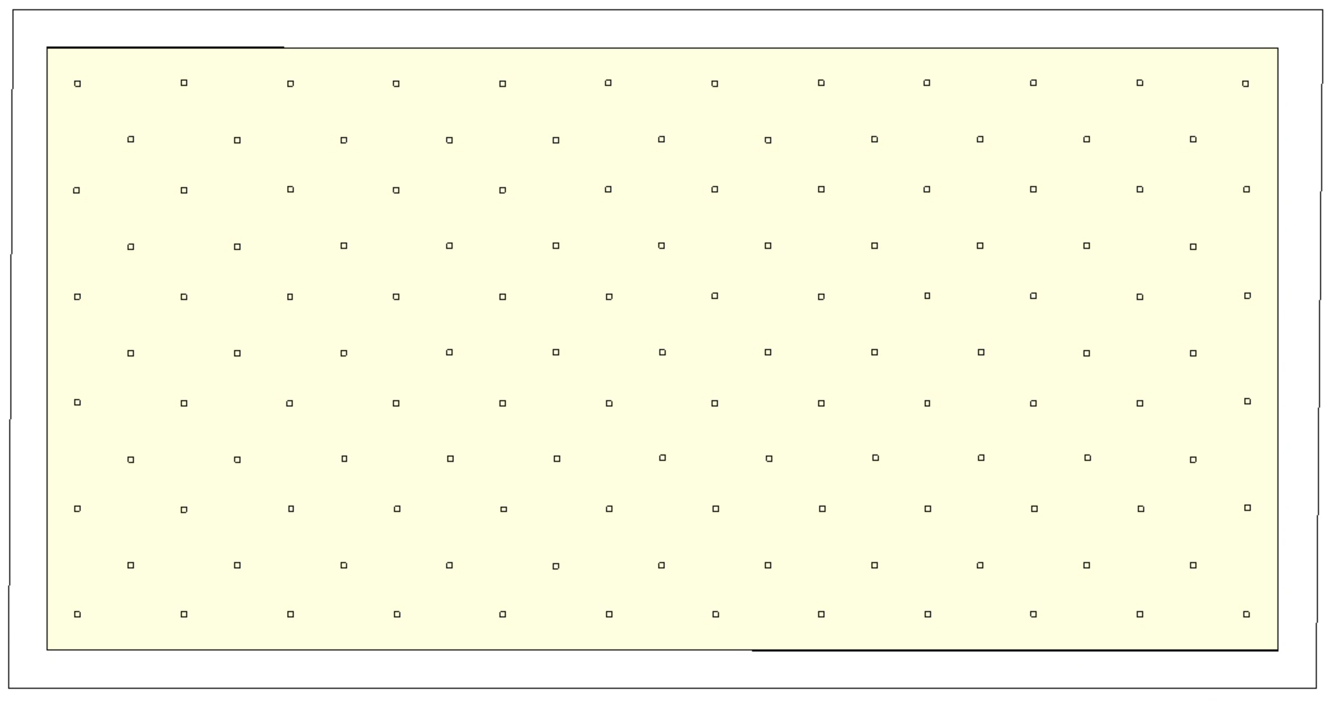
Figure 1: Centered Square COB LED Arrangement.

Uniform-Matrix Gen 2 System

Samsung SI-B8T502560WW modules are placed in a standard rectangular matrix layout, commonly used in commercial applications.

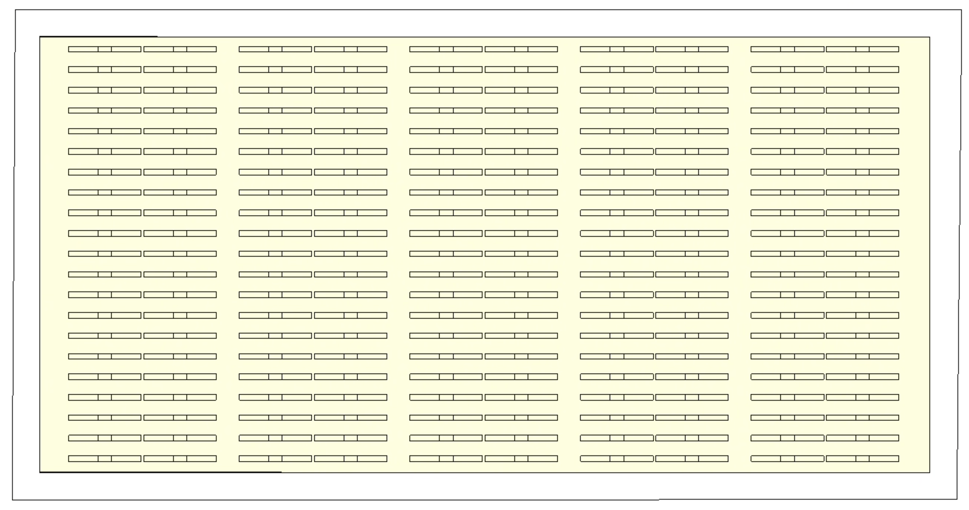
Figure 2: Uniform Matrix Arrangement of Gen 2 Modules.

Simulation Approach

Photometric data (.ies files), geometric arrangements, and surface reflectances were used in DIALux to simulate lux distributions. Results were then converted to PPFD using Spectral Power Distribution (SPD)-derived conversion factors.

Lux to PPFD Conversion

The conversion from illuminance (lux) to photosynthetic photon flux density (PPFD, in μmol m⁻² s⁻¹) uses the LED’s normalized spectral power distribution I(λ) over a wavelength range [λ₁, λ₂]. In our approach, PPFD is calculated as:

\[ \text{PPFD} = \frac{10^6}{N_A \, h \, c} \int_{\lambda_1}^{\lambda_2} I(\lambda)\,\bigl(\lambda\times10^{-9}\bigr)\,d\lambda \]

where:

h is Planck’s constant,
c is the speed of light,
N_A is Avogadro’s number,
the factor 10⁶ converts moles to micromoles,
and the λ×10⁻⁹ term converts nanometers to meters.

Illuminance, E (in lux), is given by:

\[ E = 683 \int_{\lambda_1}^{\lambda_2} I(\lambda)\,V(\lambda)\,d\lambda \]

where V(λ) is the CIE photopic luminous efficiency function and 683 lux W⁻¹ is the maximum luminous efficacy of radiation.

Therefore, the lux-to-PPFD conversion factor, C (in μmol m⁻² s⁻¹ lux⁻¹), is:

\[ C = \frac{\text{PPFD}}{E} = \frac{\displaystyle\frac{10^6}{N_A \, h \, c} \int_{\lambda_1}^{\lambda_2} I(\lambda)\,\bigl(\lambda\times10^{-9}\bigr)\,d\lambda} {683 \displaystyle \int_{\lambda_1}^{\lambda_2} I(\lambda)\,V(\lambda)\,d\lambda} \]

Conversion factors used:

Samsung Gen 2: 0.0179 μmol m⁻² s⁻¹ lux⁻¹
Samsung COB: 0.0138 μmol m⁻² s⁻¹ lux⁻¹

Results

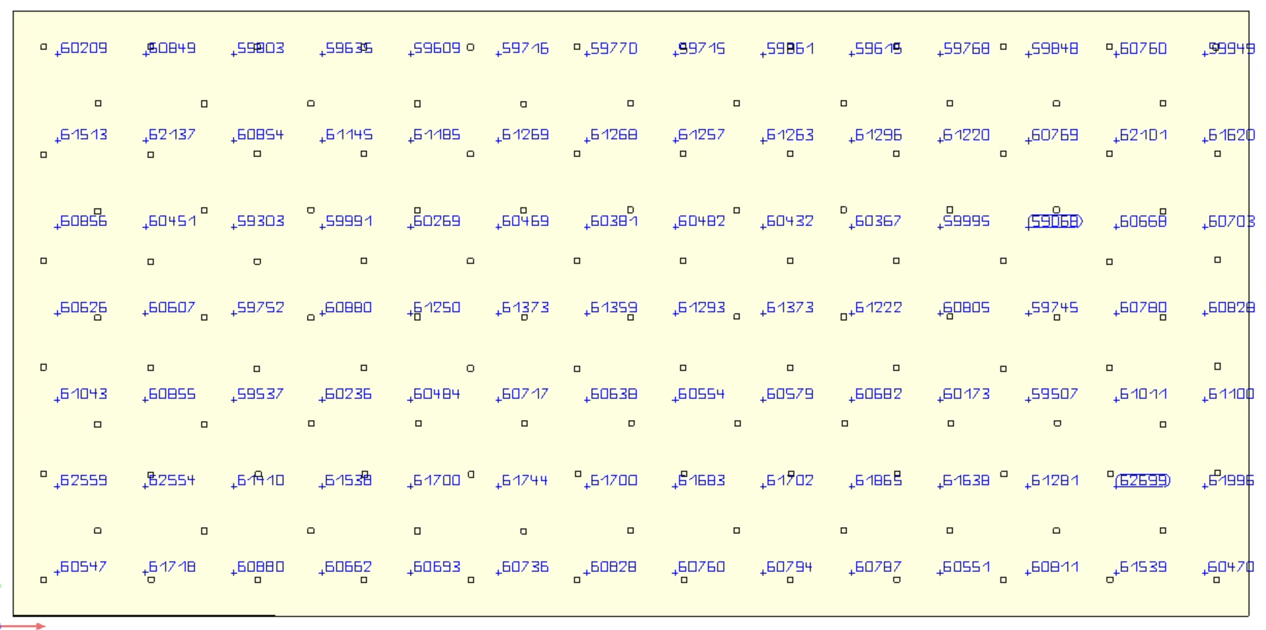
Figure 3: Novel System PAR Map

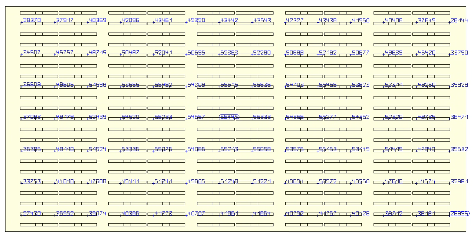
Figure 4: Conventional System PAR Map

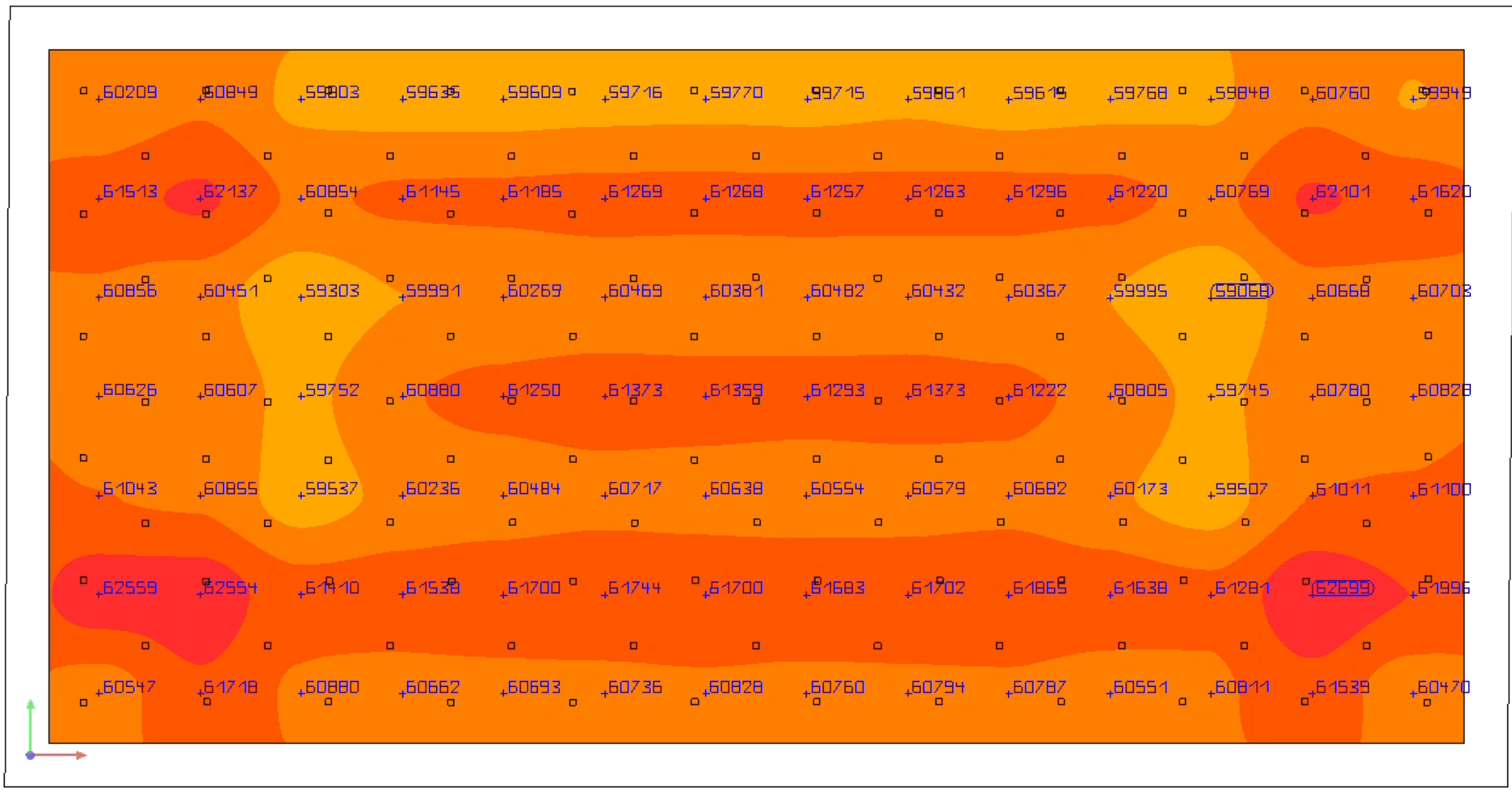
Figure 5: Novel System Heatmap

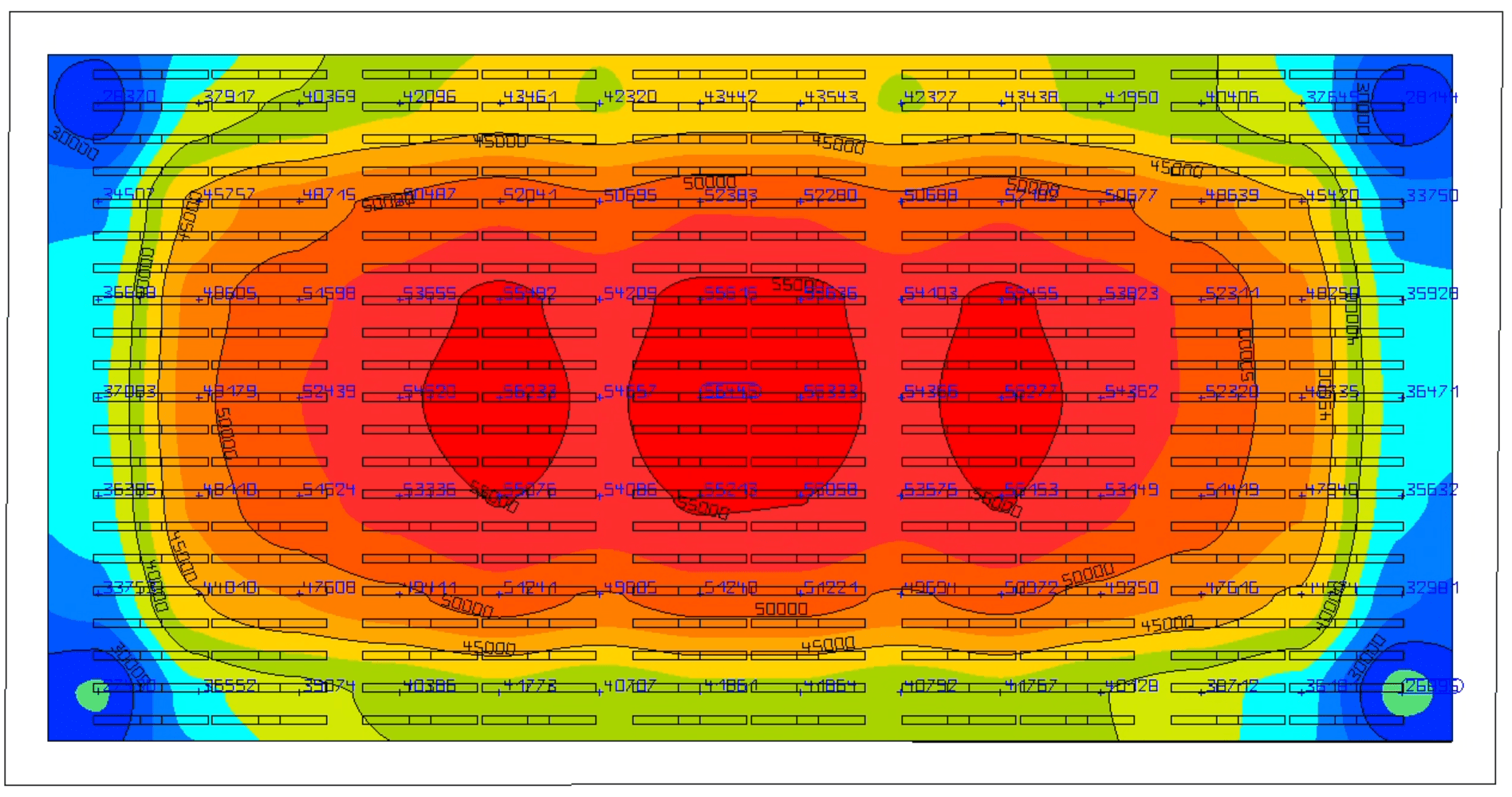
Figure 6: Conventional System Heatmap

**Simulation Metrics**
Metric	Novel System	Conventional System
Average PPFD	838.98	830.55
RMSE	10.28	138.10
DOU (%)	98.77	83.37
MAD	7.99	119.40
CV (%)	1.23	16.63
Min/Max PPFD	0.94	0.48

Mathematical Representation of Metrics

Here, we define the mathematical formulations used to calculate the metrics presented in the table above. Let P_i represent the PPFD value at the i-th measurement point, and let n be the total number of measurement points (here, n = 98).

Average PPFD (PPFD_avg):
\[ \text{PPFD}_{\text{avg}} \;=\; \frac{1}{n} \sum_{i=1}^{n} P_i \]
Root Mean Squared Error (RMSE):
\[ \text{RMSE} \;=\; \sqrt{\frac{1}{n} \sum_{i=1}^{n} \bigl(P_i - \text{PPFD}_{\text{avg}}\bigr)^2} \]
Degree of Uniformity (DOU):
\[ \text{DOU} \;=\; 100 \times \Bigl(1 - \frac{\text{RMSE}}{\text{PPFD}_{\text{avg}}}\Bigr) \]
Mean Absolute Deviation (MAD):
\[ \text{MAD} \;=\; \frac{1}{n} \sum_{i=1}^{n} \bigl|P_i - \text{PPFD}_{\text{avg}}\bigr| \]
Coefficient of Variation (CV):
CV is the ratio of the standard deviation (σ) to the average PPFD, expressed as a percentage. The standard deviation is:

\[ \sigma \;=\; \sqrt{\frac{1}{n} \sum_{i=1}^{n} \bigl(P_i - \text{PPFD}_{\text{avg}}\bigr)^2} \]

Thus

\[ \text{CV} \;=\; 100 \times \frac{\sigma}{\text{PPFD}_{\text{avg}}} \]

Note: Since we use all data points, population and sample standard deviations coincide.