Horticultural Lighting Simulation: Deep Dive
This page provides a detailed explanation of the mathematical models, algorithms, and implementation of our advanced lighting simulation script. We focus on a physics-based approach, using radiosity to accurately model light distribution in controlled-environment agriculture.
1. Introduction
Accurate prediction of Photosynthetic Photon Flux Density (PPFD) is critical for optimizing plant growth and energy efficiency in indoor farming. Our simulation script moves beyond simple direct irradiance calculations by incorporating a patch-based radiosity method. This allows us to model the complex interplay of light reflections within a grow space, leading to significantly more accurate results.
2. Methodology
2.1. Lambertian Emission Model
Chip-on-Board (COB) LEDs, a common choice for horticultural lighting, are well-approximated by a Lambertian emission pattern. This means that the radiant intensity \(I(\theta)\) varies with the cosine of the angle \(\theta\) from the LED's normal (the direction it's pointing):
\[ I(\theta) = I_0 \cos(\theta) \]
Where \( I_0 \) is the intensity along the normal (\(\theta = 0\)).
The direct irradiance \(E\) at a point on the floor from a single LED, assuming the LED is pointing straight down, is given by:
\[ E = \frac{P}{\pi} \cdot \frac{\cos(\theta)}{r^2} = \frac{P}{\pi} \cdot \frac{z}{r^3} \]
Where:
- \(P\) is the radiant flux of the LED (in Watts).
- \(z\) is the vertical distance from the LED to the floor.
- \(r\) is the total distance from the LED to the point on the floor. \(\theta\) and \(r\) are related by: \(r = \sqrt{x^2 + y^2 + z^2}\) where \(x\) and \(y\) are the horizontal distances. And \(\cos(\theta) = z/r \)).
def calculate_direct_irradiance(light_positions, light_fluxes, X, Y, H, luminous_efficacy):
    """Calculates the direct irradiance on the floor from a set of LEDs.

    Args:
        light_positions (list of tuples): (x, y, z) coordinates of each LED.
        light_fluxes (list): Luminous flux (lumens) of each LED.
        X (np.ndarray): 2D array of x-coordinates of the floor grid.
        Y (np.ndarray): 2D array of y-coordinates of the floor grid.
        H (float): Height of the LEDs above the floor.
        luminous_efficacy (float): Luminous efficacy (lm/W) of the LEDs.

    Returns:
        np.ndarray: 2D array of direct irradiance values (W/m²) on the floor.
    """
    direct_irr = np.zeros_like(X, dtype=np.float64)
    for (pos, lum) in zip(light_positions, light_fluxes):
        P = lum / luminous_efficacy  # Radiant flux (W)
        x0, y0, z0 = pos
        dx = X - x0
        dy = Y - y0
        dz = -z0  # Floor is at z=0
        dist2 = dx*dx + dy*dy + dz*dz
        dist = np.sqrt(dist2)

        with np.errstate(divide='ignore', invalid='ignore'):
            cos_th = -dz / dist  # Cosine of angle
        cos_th[cos_th < 0] = 0  # Only downward light
        with np.errstate(divide='ignore'):
            E = (P / math.pi) * (cos_th / dist2)
        direct_irr += np.nan_to_num(E)  # Accumulate irradiance
    return direct_irr
2.2. Patch-Based Radiosity
2.2.1. Surface Subdivision
The core of the radiosity method is dividing the surfaces of the room (walls, ceiling, and floor) into smaller patches. This allows us to model the non-uniform distribution of reflected light. Our script uses rectangular patches.
def subdivide_wall(x0, y0, z0, width, height, nx, ny, normal):
    """Subdivides a wall into rectangular patches.

    Args:
        x0, y0, z0: Coordinates of the bottom-left corner of the wall.
        width: Width of the wall.
        height: Height of the wall.
        nx: Number of subdivisions along the width.
        ny: Number of subdivisions along the height.
        normal: Normal vector of the wall (tuple).

    Returns:
        list: List of patch centers (tuples), list of patch areas,
              list of patch normals.
    """
    patch_centers = []
    patch_areas = []
    patch_normals = []
    dx = width / nx
    dy = height / ny
    area = dx * dy
    for i in range(nx):
        for j in range(ny):
            cx = x0 + (i + 0.5) * dx
            cy = y0 + (j + 0.5) * dy
            cz = z0
            patch_centers.append((cx, cy, cz))
            patch_areas.append(area)
            patch_normals.append(normal)
    return patch_centers, patch_areas, patch_normals

# Example usage for the wall at x=0:
wall_x0_centers, wall_x0_areas, wall_x0_normals = subdivide_wall(
    0, 0, 0, L, H, WALL_SUBDIVS_X, WALL_SUBDIVS_Y, (-1, 0, 0)
)
2.2.2. Form Factor Calculation
The form factor \(F_{ij}\) between two patches \(i\) and \(j\) quantifies the fraction of energy leaving patch \(i\) that directly reaches patch \(j\). It depends on the geometry and orientation of the patches. For small, diffuse, rectangular patches, we use the following approximation:
\[ F_{ij} = \frac{\cos(\theta_i) \cos(\theta_j) A_j}{\pi r^2} \]
Where:
- \(\theta_i\) is the angle between the normal of patch \(i\) and the direction vector from patch \(i\) to patch \(j\).
- \(\theta_j\) is the angle between the normal of patch \(j\) and the direction vector from *patch j to patch i*.
- \(A_j\) is the area of patch \(j\).
- \(r\) is the distance between the centers of patch \(i\) and patch \(j\).
If either \(\cos(\theta_i)\) or \(\cos(\theta_j)\) is negative, the patches do not "see" each other, and \(F_{ij} = 0\). Note that \(F_{ij}\) is *not* generally equal to \(F_{ji}\) because of the area term (\(A_j\)).
def calculate_form_factor(patch_center_i, normal_i, patch_center_j, normal_j, area_j):
    """Calculates the form factor between two patches.

    Args:
        patch_center_i: Center of patch i (tuple).
        normal_i: Normal vector of patch i (tuple).
        patch_center_j: Center of patch j (tuple).
        normal_j: Normal vector of patch j (tuple).
        area_j: Area of patch j (float).

    Returns:
        float: The form factor F_ij, or 0 if patches don't "see" each other.
    """
    dd = np.array(patch_center_j) - np.array(patch_center_i) #vector from i to j
    dist2 = np.dot(dd, dd)
    if dist2 < 1e-12:  # Avoid division by zero (same patch)
        return 0.0
    dist = np.sqrt(dist2)
    cos_i = np.dot(normal_i, dd) / (dist * np.linalg.norm(normal_i))
    cos_j = np.dot(normal_j, -dd) / (dist * np.linalg.norm(normal_j)) #note the -dd

    if cos_i < 0 or cos_j < 0:
        return 0.0  # Patches do not "see" each other

    ff = (cos_i * cos_j * area_j) / (math.pi * dist2)
    return ff
2.2.3. Radiosity Equation and Iterative Solution
The radiosity \(B_i\) of a patch \(i\) is the total radiant energy leaving that patch per unit area. It's the sum of the emitted energy \(E_i\) (which is zero for non-emitting surfaces like walls and floor) and the reflected energy:
\[ B_i = E_i + \rho_i \sum_{j=1}^{N} F_{ij} B_j \]
Where:
- \(E_i\) is the emitted radiosity of patch \(i\) (zero for non-light sources).
- \(\rho_i\) is the reflectance of patch \(i\).
- \(F_{ij}\) is the form factor from patch \(i\) to patch \(j\).
- \(B_j\) is the radiosity of patch \(j\).
- \(N\) is the total number of patches.
This is a system of linear equations that can be solved iteratively. Our script uses a simple iterative approach (similar to the Jacobi method):
- Initialization: Initialize the radiosity of each patch. For light-emitting patches (LEDs), this initial radiosity is based on their radiant flux. For non-emitting patches, the initial radiosity is zero.
- Iteration:
- For each patch \(i\), calculate the total incoming flux from all other patches: \(\sum_{j=1}^{N} F_{ij} B_j A_j\) (where \(A_j\) is the area of patch j).
- Update the radiosity of patch \(i\): \(B_i^{new} = E_i + \rho_i \frac{\sum_{j=1}^{N} F_{ij} B_j A_j}{A_i}\). We divide by the receiving patch's area \(A_i\) to get the radiosity (energy per unit area) from the incoming flux.
- Repeat: Repeat step 2 for a specified number of iterations (`NUM__RADIOSITY__BOUNCES`) or until the radiosity values converge.
def calculate_radiosity(patch_centers, patch_areas, patch_normals, patch_refl,
                       light_positions, light_fluxes, luminous_efficacy, num_bounces):
    """Calculates the radiosity of each patch using an iterative method.

    Args:
        patch_centers: List of patch center coordinates (tuples).
        patch_areas: List of patch areas (floats).
        patch_normals: List of patch normal vectors (tuples).
        patch_refl: List of patch reflectances (floats).
        light_positions: List of LED positions (tuples).
        light_fluxes: List of LED luminous fluxes (lumens).
        luminous_efficacy: Luminous efficacy (lm/W).
        num_bounces: Number of radiosity bounces.

    Returns:
        np.ndarray: Array of radiosity values for each patch.
    """
    Np = len(patch_centers)
    patch_rad = np.zeros(Np)

    # 1. Initialize radiosity (direct irradiance on patches)
    patch_direct = np.zeros(Np)
    for ip in range(Np):
      pc = patch_centers[ip]
      n = patch_normals[ip]
      accum = 0.0
      for (lp, lum) in zip(light_positions, light_fluxes):
        P = lum/luminous_efficacy
        dx = pc[0]-lp[0]
        dy = pc[1]-lp[1]
        dz = pc[2]-lp[2]
        dist2 = dx*dx + dy*dy + dz*dz
        if dist2<1e-12:
          continue
        dist = math.sqrt(dist2)

        dd = np.array([dx, dy, dz])
        dist = np.linalg.norm(dd)
        cos_th_led = -dz/dist
        if cos_th_led < 0:
          # patch is "above" LED or sideways
          continue
        E_led = (P/math.pi)*(cos_th_led/(dist2))

        # Now cos_in on the patch side:
        cos_in_patch = np.dot(-dd, n)/(dist*np.linalg.norm(n))
        if cos_in_patch<0:
          cos_in_patch=0
        accum+=E_led*cos_in_patch
      patch_direct[ip] = accum
    patch_rad = patch_direct

    # 2. Iterative radiosity calculation
    for bounce in range(num_bounces):
        new_flux = np.zeros(Np)  # Accumulated flux *received* by each patch
        for j in range(Np):
            if patch_refl[j] <= 0:  # Skip non-reflective patches
                continue
            # Outgoing flux from patch j
            outF = patch_rad[j] * patch_areas[j] * patch_refl[j]
            # Distribute flux to other patches
            for i in range(Np):
                if i == j:
                    continue  # Skip self
                ff = calculate_form_factor(patch_centers[j], patch_normals[j],
                                          patch_centers[i], patch_normals[i],
                                          patch_areas[i])  # Use area of *receiving* patch
                new_flux[i] += outF * ff  # Flux received by patch i

        # 3. Update radiosity values
        patch_rad = patch_direct + new_flux / patch_areas  # Add reflected

    return patch_rad
2.3. Calculating PPFD on the Floor
Once the radiosity of all patches is calculated, the total irradiance (direct + reflected) at any point on the floor can be determined. The direct irradiance is calculated using the Lambertian emission model (as described in Section 2.1). The reflected irradiance is calculated by summing the contributions from all reflecting patches:
\[E_{reflected} = \sum_{i=1}^{N} B_i A_i F_{i,floor} \]
where:
- \(B_i\) is the radiosity of patch \(i\).
- \(A_i\) is the area of patch \(i\).
- \(F_{i,floor}\) is the form factor from patch \(i\) to the point on the floor. This is calculated using the same formula as before, but now one "patch" is a point on the floor.
Finally, the total irradiance is converted to PPFD using the conversion factor derived from the SPD data.
def calculate_floor_ppfd(X, Y, patch_centers, patch_areas, patch_normals,
                         patch_rad, patch_refl, light_positions, light_fluxes,
                         luminous_efficacy, conversion_factor):
    """Calculates the total PPFD (direct + reflected) on the floor.
    """
    # 1. Direct irradiance (already calculated in previous examples)
    direct_irr = calculate_direct_irradiance(light_positions, light_fluxes,
                                            X, Y, H, luminous_efficacy)

    # 2. Reflected irradiance
    reflect_irr = np.zeros_like(X, dtype=np.float64)
    floor_pts = np.stack([X.ravel(), Y.ravel(), np.zeros_like(X.ravel())], axis=1)
    floor_n = np.array([0, 0, 1], dtype=float)  # Normal of the floor

    for p in range(len(patch_centers)):
        outF = patch_rad[p] * patch_areas[p] * patch_refl[p]
        if outF < 1e-15:  # Skip negligible contributions
            continue
        pc = patch_centers[p]
        n = patch_normals[p]
        dv = floor_pts - pc  # Vector from patch to floor points
        dist2 = np.einsum('ij,ij->i', dv, dv) # Efficient distance calculation
        dist = np.sqrt(dist2)
        cos_p = np.einsum('ij,j->i', dv, n) / (dist * np.linalg.norm(n) + 1e-15)
        cos_f = np.einsum('ij,j->i', -dv, floor_n) / (dist + 1e-15)
        cos_p[cos_p < 0] = 0
        cos_f[cos_f < 0] = 0
        ff = (cos_p * cos_f) / (math.pi * dist2 + 1e-15) #form factor to floor *point*
        cell_flux = outF * ff
        cell_area = FLOOR_GRID_RES * FLOOR_GRID_RES #grid size on floor
        cell_irr = cell_flux / cell_area
        reflect_irr.ravel()[:] += np.nan_to_num(cell_irr) # Accumulate

    # 3. Total irradiance and PPFD
    floor_irr = direct_irr + reflect_irr
    floor_ppfd = floor_irr * conversion_factor
    return floor_ppfd
3. Results and Visualization
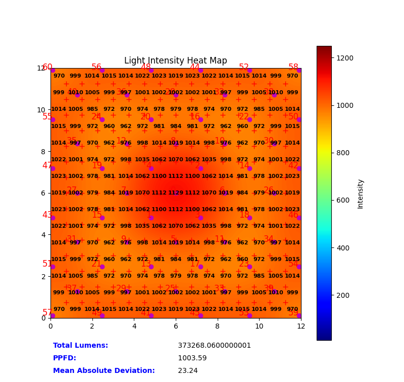
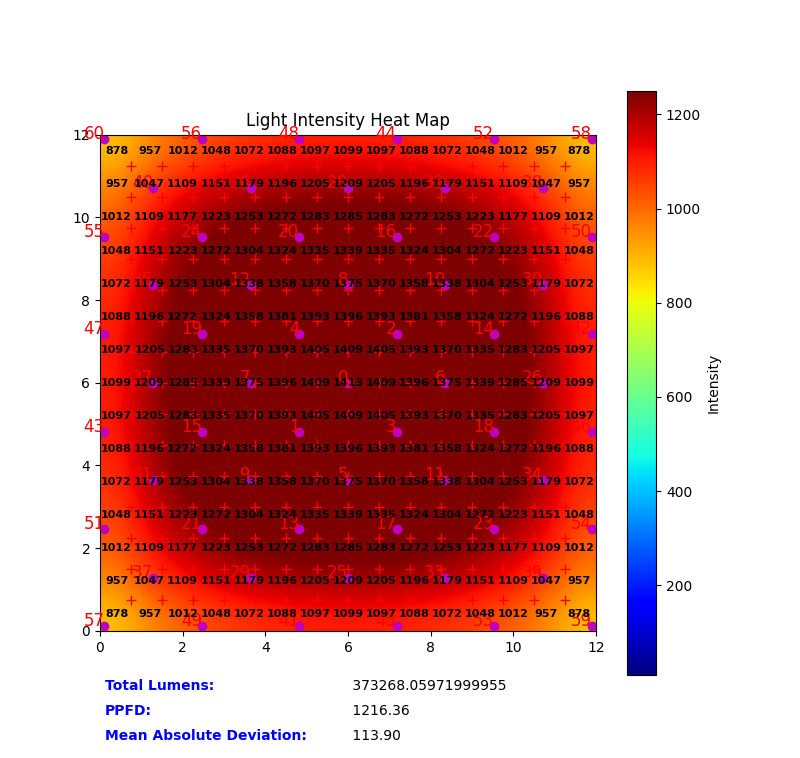
The script outputs a heatmap visualizing the PPFD distribution on the floor. This allows for a clear visual assessment of lighting uniformity. Key metrics are also calculated:
- Average PPFD: The average PPFD value across the floor.
- Mean Absolute Deviation (MAD): A measure of deviation of the PPFD from the average PPFD. Lower MAD indicates better uniformity.
- Degree of Uniformity (DOU): A percentage representing the uniformity of the PPFD distribution, calculated as:
\(DOU = 100 \times (1 - \frac{MAD}{Average PPFD})\)

Figure 1: Example PPFD heatmap for UPFP-based methodology generated by the simulation script. Warmer colors represent higher PPFD values.

Figure 2: Example PPFD heatmap for standard methodology generated by the simulation script. Warmer colors represent higher PPFD values.
4. Conclusion
Our lighting simulation script provides a physically accurate and computationally efficient way to model PPFD distribution in controlled-environment agriculture. The use of a patch-based radiosity method allows for a detailed analysis of light reflections, leading to more realistic results than simpler models. This tool is valuable for optimizing lighting system design, improving plant growth, and maximizing energy efficiency.

