Technology

Explore the innovative technology behind Luminous Photonics' horticultural lighting solutions, based on our Uniform Photon Flux Principle (UPFP) for modular LED arrays.

Uniform Photon Flux Principle (UPFP)

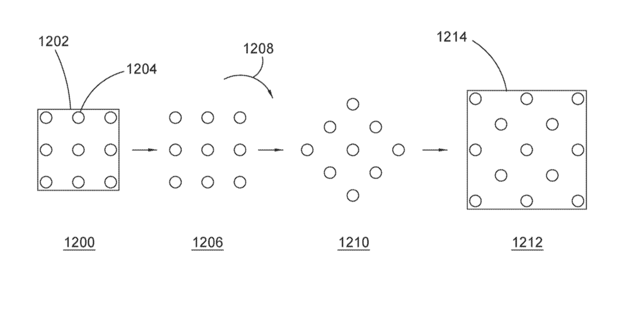
Our research has led to the development of the Uniform Photon Flux Principle (UPFP), a groundbreaking approach to optimizing Photosynthetic Photon Flux Density (PPFD) distribution in controlled-environment agriculture. The UPFP leverages a particular arrangement of Chip-on-Board (CoB) LED elements, positioned according to the centered square number integer sequence (Online Encyclopedia of Integer Sequences: A001844) pattern logic. By carefully assigning optimal intensities to each layer, as informed by our proprietary differential evolution-based global optimization algorithm, we achieve unprecedented uniformity in PPFD across the growing area.

Key Benefits of the UPFP:

Infinitely Scalable Modularized System

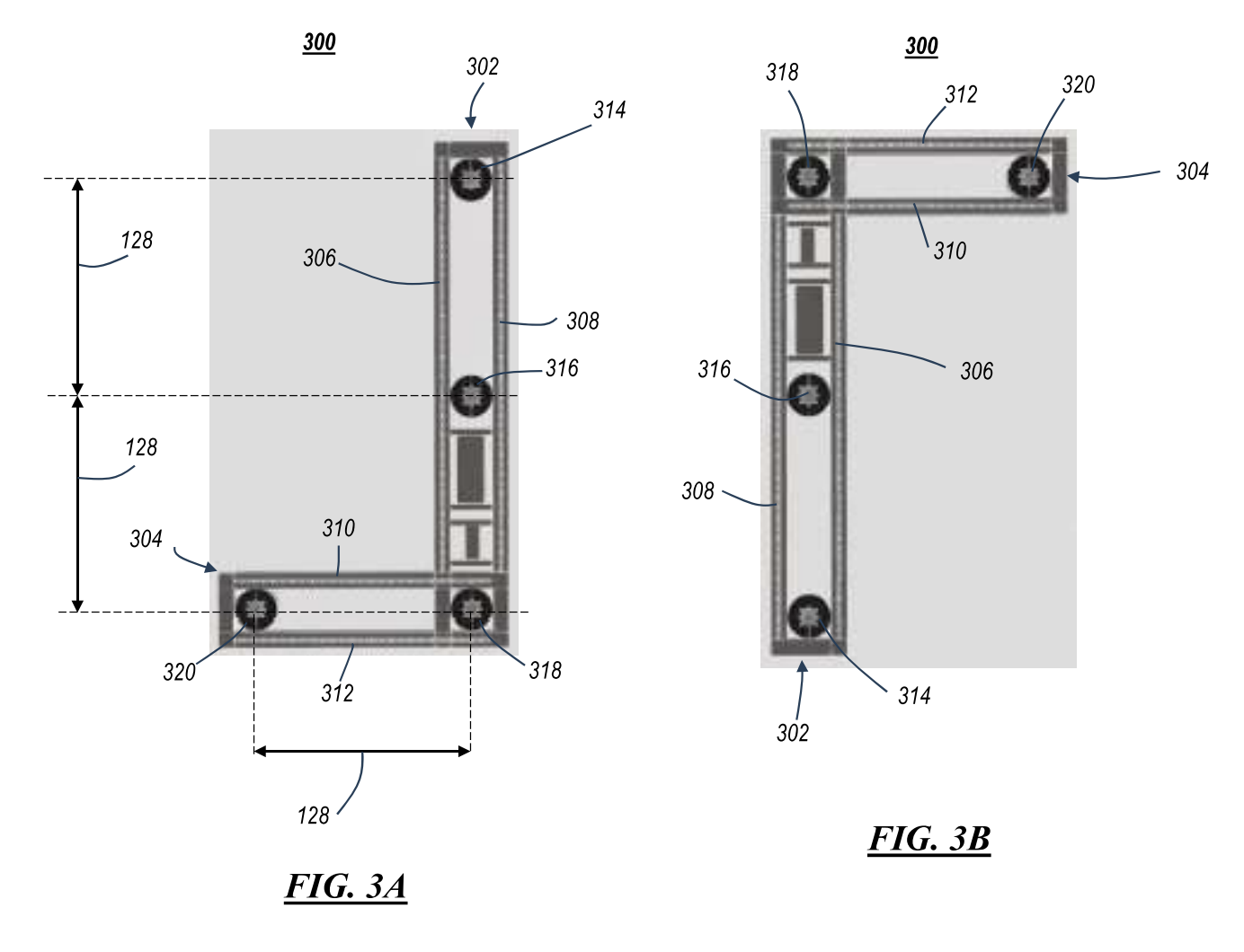
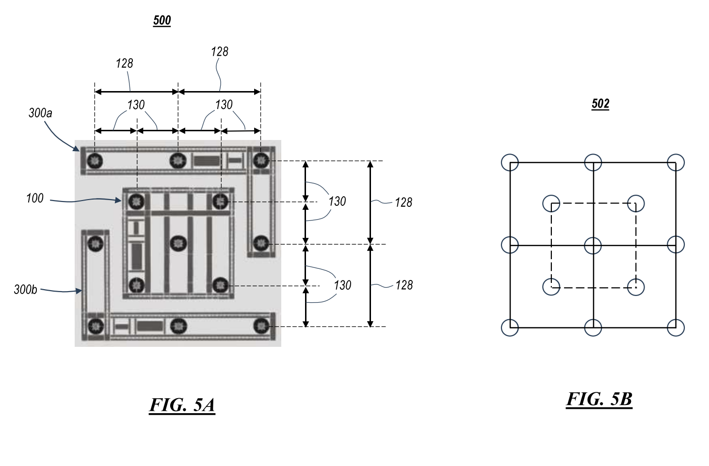
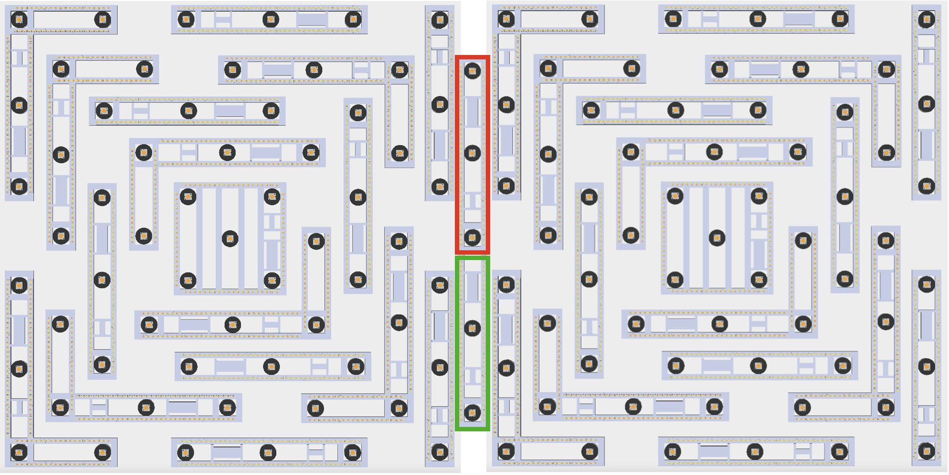
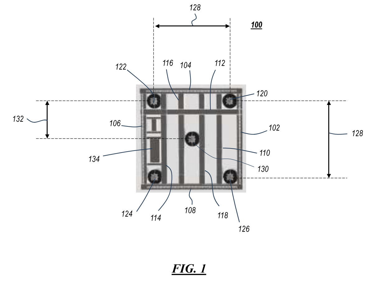
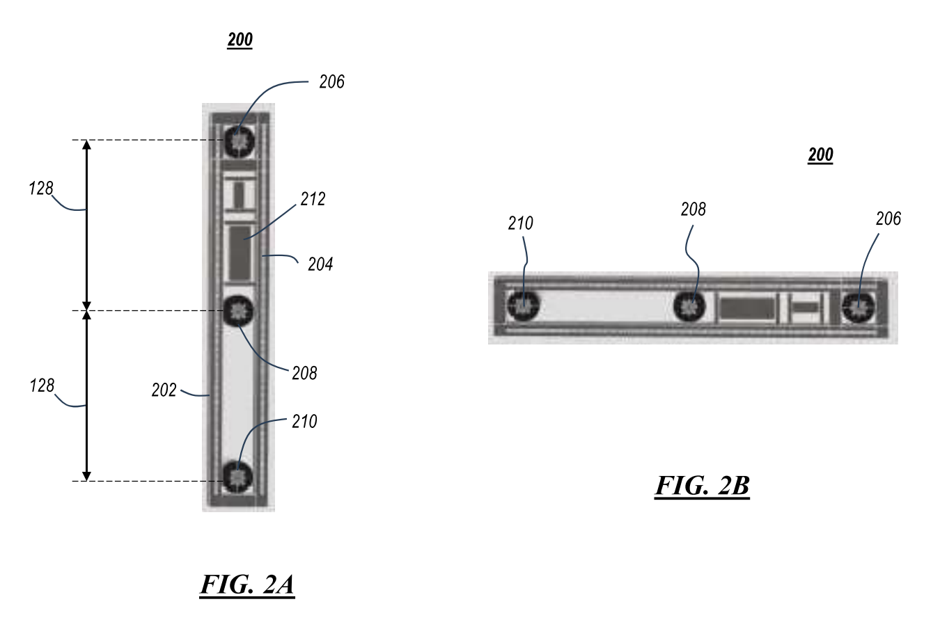
With just 4 types of modular pieces, our horticultural lighting system can optimally cover any size square or rectangular space.

Our arrangement strategem continues ad infinitum...

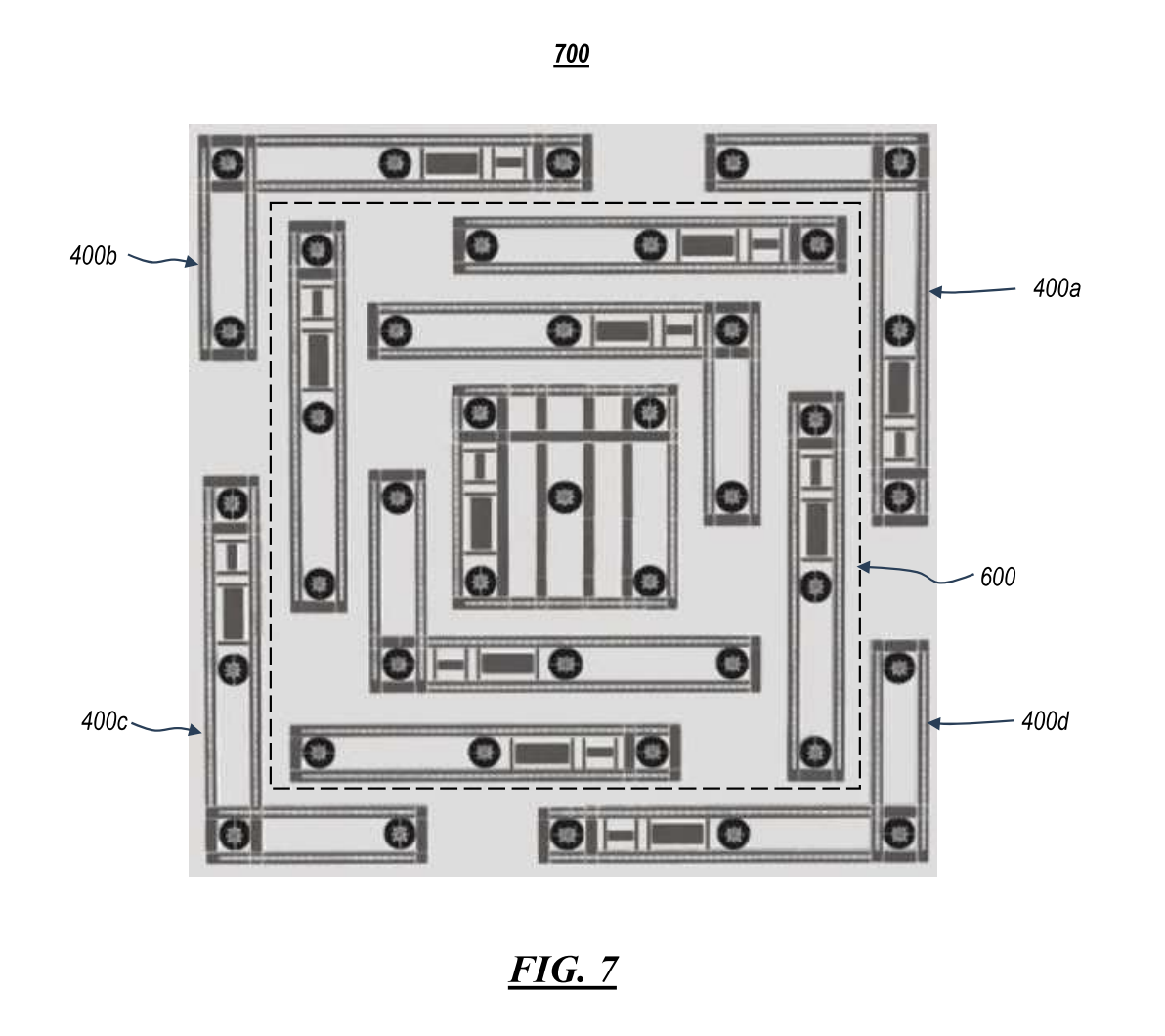
Infinite concentric square layers can be added to create endless configurations of arrays.

Here's an example of a 61-CoB lighting array.
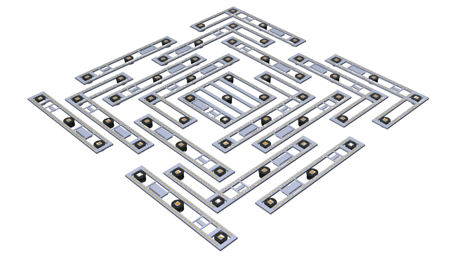
Modular Assembly #4

And with just 2 linear connector modules, two square lighting arrays can be conjoined to form a perfect rectangular lighting array.

Visualizing Light Uniformity

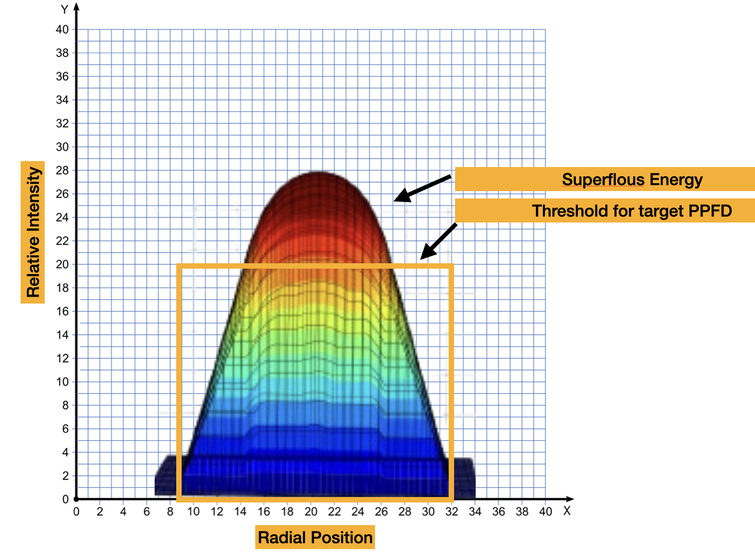
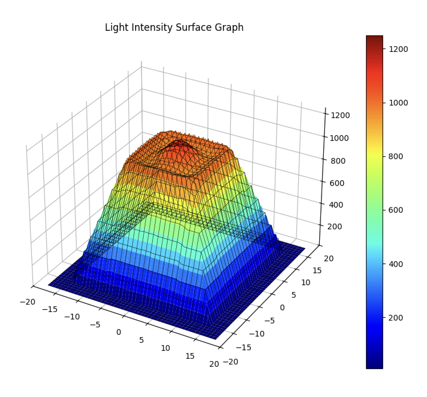
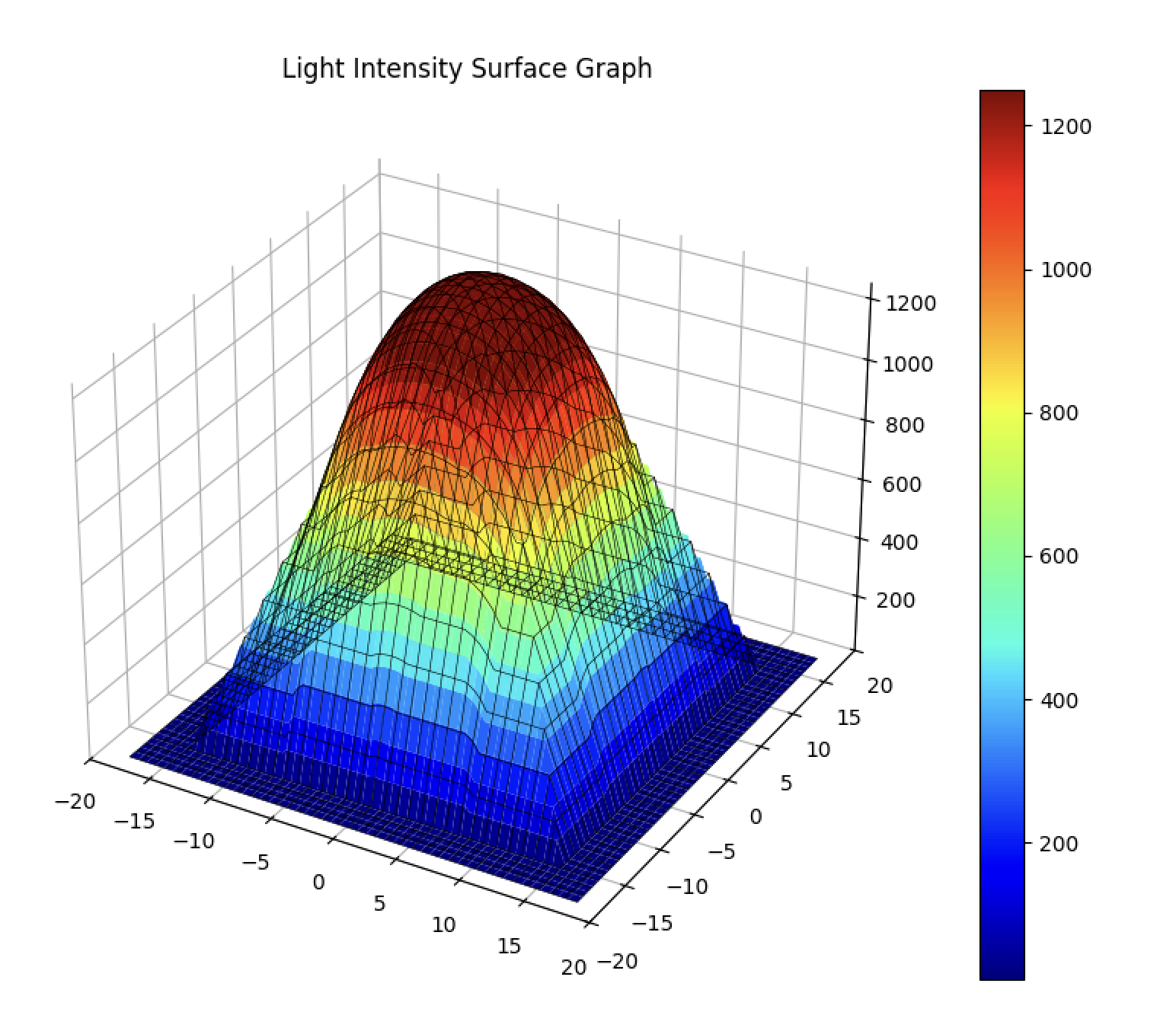
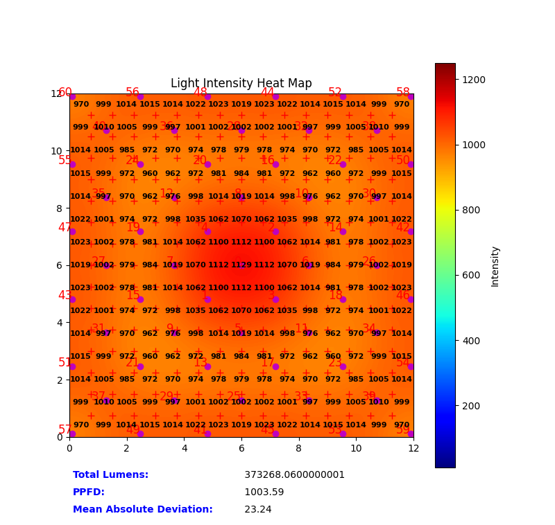
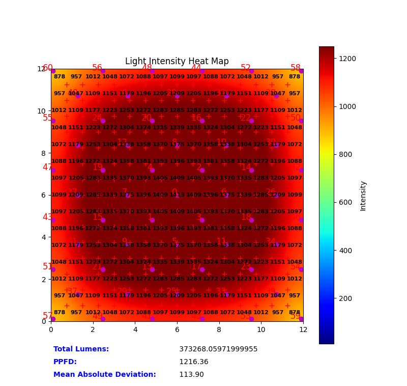
Below are graphical representations that demonstrate the effectiveness of employing the UPFP in our patented technology to achieve truly uniform light distribution. Each set of graphs offers a simple comparison to highlight our UPFP-based approach: Each simulation uses the same centered square sequence pattern arrangement of LEDs, but the graphs on the right show a simulation where the same luminous flux was applied to each LED, while the graphs on the left show layer-wise luminous flux assignments that are informed by our differential evolution-based global optimization algorithm.

Beam Profile

These graphs illustrate the spatial distribution of light intensity, highlighting the "superfluous energy" outside the target PPFD range. The UPFP-based graph on the left demonstrates a more uniform beam spread with significantly reduced energy waste.

Figure 1: Comparison of Beam Profiles. Right: Traditional distribution. Left: Optimized UPFP distribution.

PPFD Surface Graphs

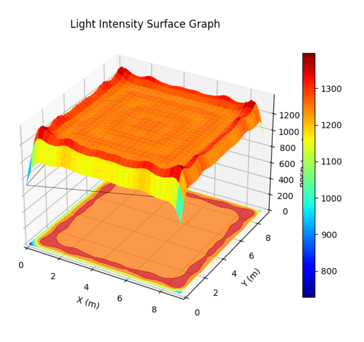
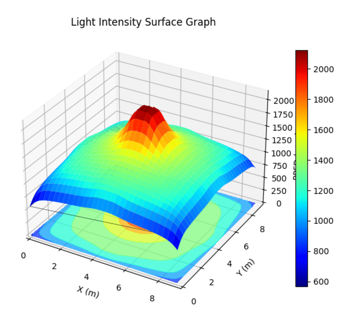
These 3D graphs illustrate the spatial distribution of PPFD, as presented in our research. The colors represent different intensity levels, with blue being low and red being high. The orange square shows the target PPFD range. Note how the UPFP-based graph on the left exhibits a more uniform distribution with minimal "superfluous energy" (light outside the target PPFD range).

Figure 2: Comparison of PPFD Surface Graphs. Right: Traditional distribution. Left: Optimized UPFP distribution.

In the surface graphs below, which represent data from a larger floor size of 30' x 30', versus the 12' x 12' floor size referenced above, it can be seen that the non-uniformity for the uniform grid matrix of LEDs with all the same luminous flux applied to the LEDs is exacerbated, while the UPFP-based methodology has increased uniformity.

Figure 3: Comparison of 30x30 PPFD Surface Graphs. Right: Traditional distribution. Left: Optimized UPFP distribution.

2D Variance Graphs

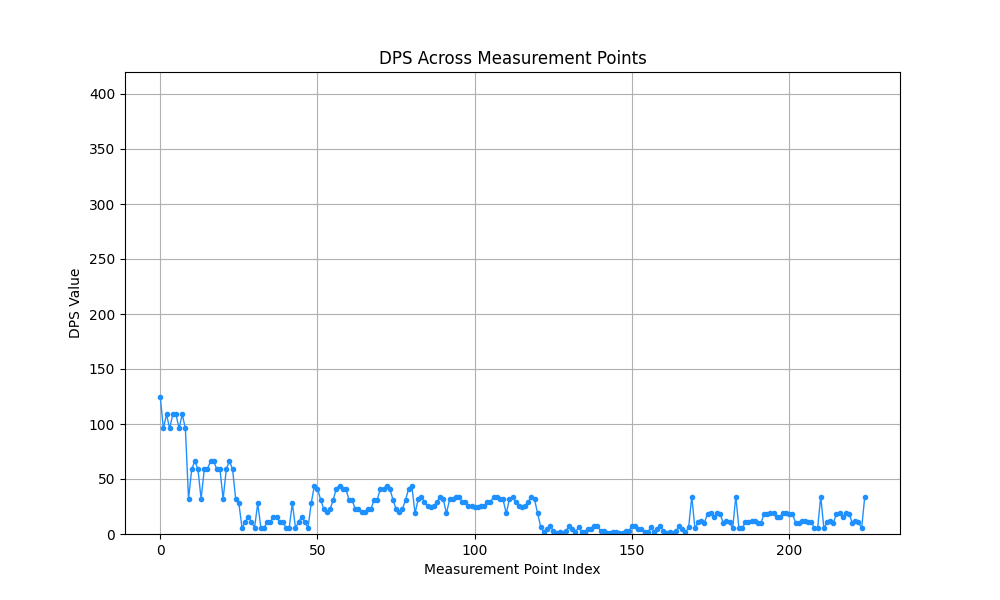
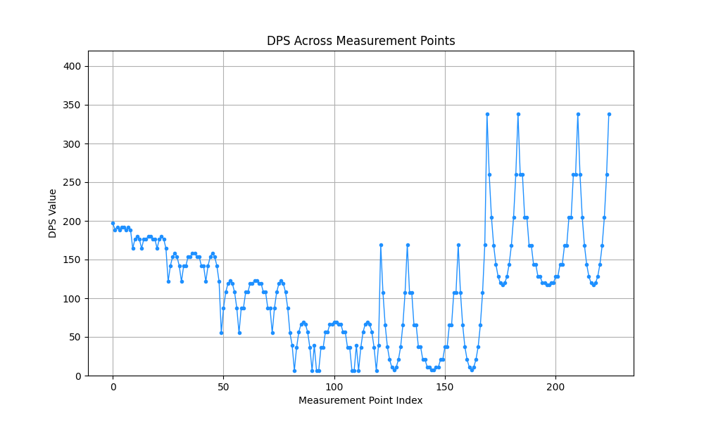
These graphs provide a top-down view of the PPFD distribution, highlighting the variance from the target PPFD. The UPFP-based approach (left) demonstrates significantly reduced variance in photon distribution, showcasing far superior uniformity.

Figure 4: Comparison of 2D Variance Graphs. Right: Traditional distribution. Left: Optimized UPFP distribution.

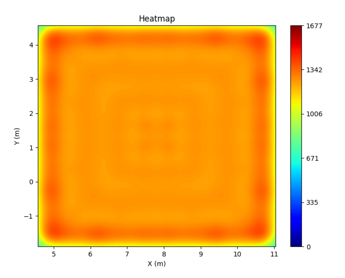
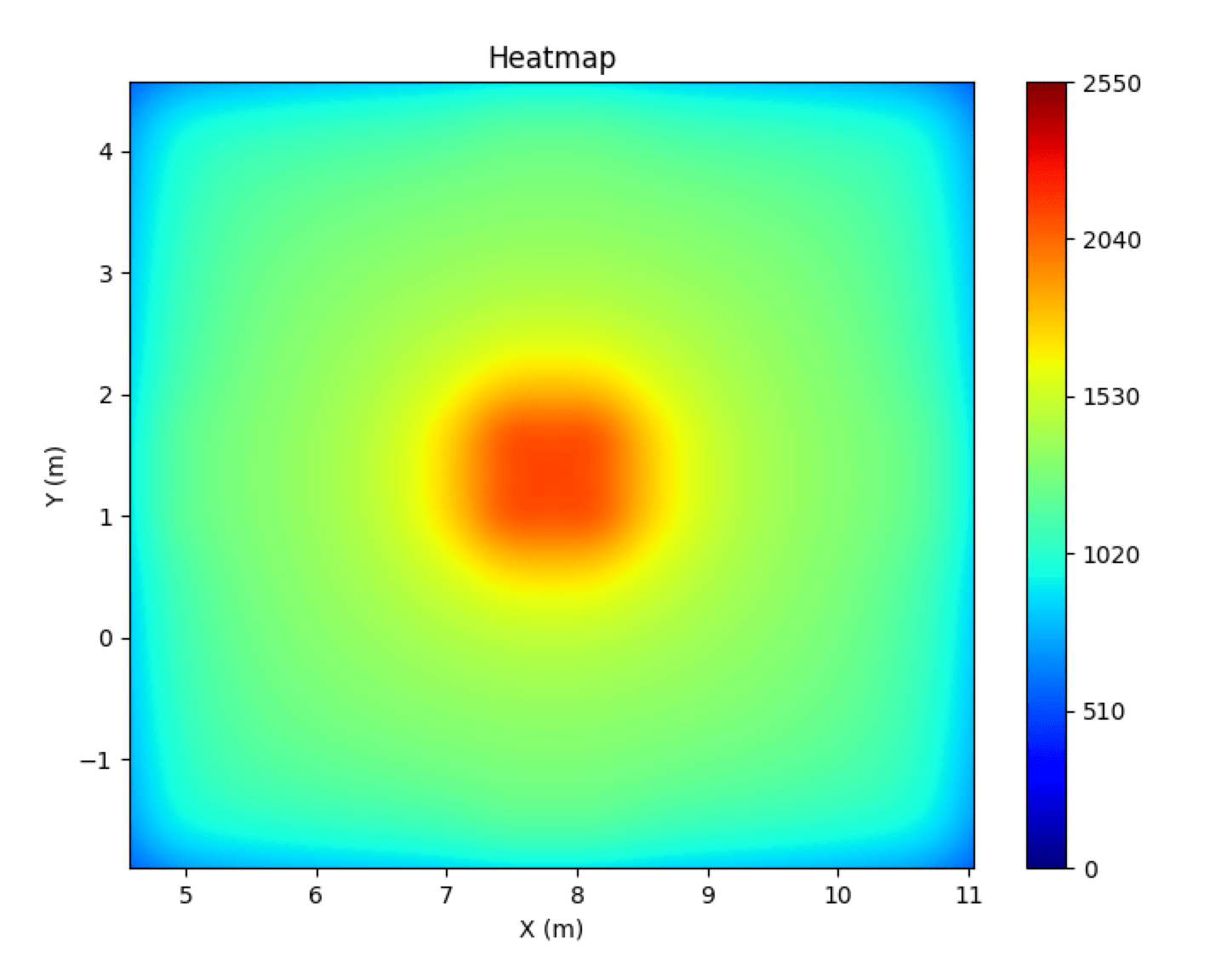
Heatmaps

Heatmaps offer another intuitive way to visualize PPFD distribution. Warmer colors (reds) represent higher PPFD, while cooler colors (blues) represent lower PPFD. The UPFP-based heatmap (left) displays a more consistent color across the growing area, signifying superior uniformity. The competitor displays a pronounced concentration of photons toward the center of the illuminated area, as can be seen by the circular radiation pattern.

Figure 5: Comparison of PPFD Heatmaps. Right: Traditional distribution. Left: Optimized UPFP distribution.

Figure 6: Comparison of 30x30 PPFD Heatmaps. Right: Traditional distribution. Left: Optimized UPFP distribution.

Dive Deeper into the Simulation
Check out a DIALux Simulation

Differential Evolution-Based Global Optimization Algorithm

Utilizing our physics-based radiosity simulation, we employ a sophisticated differential evolution-based global optimization algorithm to refine and optimize the luminous flux settings of our LED arrays. This optimization process leverages the accuracy of the radiosity model to achieve unprecedented levels of PPFD uniformity and energy efficiency.

Interact with the Algorithm

Parameterization

The optimization algorithm works with a 15-element parameter vector, representing the following:

  • COB Layer Intensities (elements 0-5): The luminous flux (in lumens) for each of the six COB LED layers in our diamond pattern arrangement.
  • LED Strip Group Intensities (elements 6-10): The luminous flux for groups of LED strips. These groups correspond to the COB layers, allowing for coordinated control.
  • Corner COB Intensities (elements 11-14): The luminous flux for the four corner COB LEDs in the outermost layer.

Objective Function

The optimization algorithm's goal is to find the set of parameters (LED intensities) that minimize an objective function. The objective function aims to minimize the Root Mean Squared Error (RMSE) between the simulated PPFD and a target PPFD, while also incorporating constraints to ensure realistic and desirable results. The objective function is defined as:

\[ \text{Objective} = w_{rmse} \cdot \text{RMSE} + w_{penalty} \cdot \text{Penalty} \]

Where:

  • \(RMSE = \sqrt{\frac{1}{N} \sum_{i=1}^{N} (PPFD_i - PPFD_{target})^2}\) is the Root Mean Squared Error between the simulated PPFD (\(PPFD_i\)) at each point on the floor grid and the target PPFD (\(PPFD_{target}\)).
  • \(\text{Penalty}\) represents additional penalty terms (described below).
  • \(w_{rmse}\) and \(w_{penalty}\) are weighting factors that control the relative importance of the RMSE and the penalty terms.

The crucial point is that calculating the RMSE requires running the full radiosity simulation with the given set of LED intensities. This is how the global optimization is linked to the physically accurate radiosity model.

Penalty Terms:

  • Degree of Uniformity (DOU) Penalty: A penalty is applied if the DOU falls below a threshold (e.g., 96%). This strongly encourages highly uniform light distribution.
  • PPFD Constraints: Nonlinear constraints (described below) ensure the average PPFD remains within a defined range (target PPFD to target PPFD + 250 µmol/m²/s).
Objective Function (Python - Simplified)

def objective_function(x, target_ppfd, fixed_base_height, rmse_weight=1.0, dou_penalty_weight=50.0):
    """
    Calculates the objective function value.

    Args:
        x (np.ndarray): The 15-element parameter vector (LED intensities).
        target_ppfd (float): The target PPFD value.
        fixed_base_height (float):  Height of the LEDs above the floor.
        rmse_weight (float): Weight for the RMSE term.
        dou_penalty_weight (float): Weight for the DOU penalty.

    Returns:
        float: The objective function value.
    """
    avg_ppfd, rmse, dou = simulate_lighting(x, fixed_base_height, plot_result=False)
    penalty = 0.0
    if dou < 96:
        penalty = dou_penalty_weight * (96 - dou)**2
    obj_val = rmse_weight * rmse + penalty
    print(f"Obj: {obj_val:.3f} | RMSE: {rmse:.3f}, DOU: {dou:.3f}, Penalty: {penalty:.3f}") #Optional Print Statement
    return obj_val
                

Global Optimization Algorithm: Differential Evolution

We use the Differential Evolution (DE) algorithm, a powerful global optimization method, to minimize the objective function. DE is well-suited for this task because:

  • Handles Non-Convexity: The objective function is likely non-convex (meaning it has multiple local minima), and DE is robust to this. Simpler gradient-based methods might get stuck in local minima.
  • Handles Constraints: DE can handle the nonlinear constraints on the average PPFD.
  • Derivative-Free: DE does not require calculating derivatives of the objective function. This is important because calculating the derivative of the radiosity simulation would be extremely complex.

The `scipy.optimize.differential_evolution` function from the SciPy library is used to perform the optimization. We define bounds for each parameter (minimum and maximum luminous flux for each LED) and nonlinear constraints to keep the average PPFD within the desired range.

Global Optimization with Differential Evolution (Python)

from scipy.optimize import differential_evolution, NonlinearConstraint

def constraint_lower(x, target_ppfd, fixed_base_height):
    avg_ppfd, _, _ = simulate_lighting(x, fixed_base_height, plot_result=False)
    return avg_ppfd - target_ppfd  # Must be >= 0

def constraint_upper(x, target_ppfd, fixed_base_height):
    avg_ppfd, _, _ = simulate_lighting(x, fixed_base_height, plot_result=False)
    return target_ppfd + 250 - avg_ppfd  # Must be >= 0

def optimize_lighting_global(target_ppfd, fixed_base_height):
    """
    Use differential evolution for global optimization.
    """
    bounds = [(1000.0, 15000.0)] * 15  # Bounds for each parameter
    nc_lower = NonlinearConstraint(lambda x: constraint_lower(x, target_ppfd, fixed_base_height), 0, np.inf)
    nc_upper = NonlinearConstraint(lambda x: constraint_upper(x, target_ppfd, fixed_base_height), 0, np.inf)
    constraints = [nc_lower, nc_upper]
    result = differential_evolution(
        lambda x: objective_function(x, target_ppfd, fixed_base_height),
        bounds,
        constraints=constraints,
        maxiter=1000,
        popsize=15,
        recombination=0.7,
        disp=True  # Display progress
    )
    return result
                

Key elements of this code:

  • `bounds`: Defines the minimum and maximum allowed luminous flux for each LED.
  • `constraints`: Defines nonlinear constraints using `NonlinearConstraint`. These ensure the average PPFD stays within the desired range (target to target + 250). The `constraint_lower` and `constraint_upper` functions are used to define these.
  • `differential_evolution`: This function performs the optimization. Key parameters include:
    • `maxiter`: The maximum number of iterations.
    • `popsize`: The population size (number of candidate solutions evolved in parallel).
    • `recombination`: A parameter controlling the mutation strategy.
    • `disp`: Set to `True` to display progress information during optimization.

Integration with Radiosity

The global optimization algorithm works by repeatedly calling the `simulate_lighting` function (which contains the full radiosity model). This is the crucial link:

  1. Initial Guess: The optimization starts with a random initial guess for the LED intensities.
  2. Radiosity Simulation: `simulate_lighting` is called with the current LED intensities. This performs the full radiosity calculation, including direct irradiance and multiple reflections, and returns the average PPFD, RMSE, and DOU.
  3. Objective Function Evaluation: The `objective_function` uses the results from `simulate_lighting` (RMSE, DOU) to calculate the objective function value.
  4. Parameter Update: The Differential Evolution algorithm uses the objective function value to update the LED intensities, creating a new set of candidate solutions.
  5. Repeat: Steps 2-4 are repeated until the algorithm converges to a solution (a set of LED intensities that minimizes the objective function).

This iterative process, combining a global optimization algorithm with a physically accurate lighting simulation, allows us to find LED settings that achieve extremely high uniformity and meet the target PPFD, even in complex room geometries.

Dive Deeper into the Radiosity Simulation

Experimental Validation

We are committed to rigorous experimental validation of our UPFP technology. We will be using Apogee Instruments spectroradiometers (PS series for lab testing and the MS-100 handheld for field testing) to empirically verify the principle across the 380–1000 nm range. These measurements will enable us to:

  • Measure total photon flux and PPFD distribution across the plant canopy.

  • Corroborate our theoretical predictions with real-world data.

  • Further refine our models and optimization algorithms.

References

  1. Zhang, G., et al., 2015. A combination of downward lighting and upward lighting improves plant growth in plant factories. Hortscience, 50(8), 1126--1130.

  2. Joshi, J., Zhang, G., Shen, S., Supaibulwatana, K., Watanabe, C., Yamori, W., 2017. A combination of downward lighting and supplemental upward lighting improves plant growth in a closed plant factory with artificial lighting. Hortscience 52 (6), 831--835. https://doi.org/10.21273/HORTSCI11822-17

  3. Kozai, T., 2022. Role and characteristics of PFALs. Plant Factory Basics, Applications and Advances, 46. Academic Press.

  4. Runkle, E., 2021. Hidden benefits of supplemental lighting. Greenhouse Product News, 42. https://gpnmag.com/article/hidden-benefits-of-supplemental-lighting/
Back to Top Home